Blending Independent Components and
Principal Components Analysis
4.2 Different blended importance criteria
[this page | pdf | references | back links]
Return to
Abstract and Contents
Next page
4.2 Different blended
importance criteria
One possible approach would be to use an importance
criterion involving a function  that includes
both variance and factors like kurtosis that characterise the extent to which
the data seems to be coming from a non-normal distribution. For example, we might
use the following:
that includes
both variance and factors like kurtosis that characterise the extent to which
the data seems to be coming from a non-normal distribution. For example, we might
use the following:
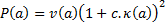
(N.B. We could also use any function that varied
monotonically in line with this function, e.g. its square root , if is positive,
and we would derive exactly the same input signals)
Here  is the variance
of the time series corresponding to the mixture of output signals characterised
by
is the variance
of the time series corresponding to the mixture of output signals characterised
by  ,
,  is its
kurtosis, and
is its
kurtosis, and  is a constant
that indicates the extent to which we want to focus on kurtosis rather than
variance in the derivation of which signals might be ‘important’. Again we
would constrain to be of ‘unit
length’, i.e. to have
is a constant
that indicates the extent to which we want to focus on kurtosis rather than
variance in the derivation of which signals might be ‘important’. Again we
would constrain to be of ‘unit
length’, i.e. to have  .
.
The larger (i.e. more positive) is,
the more we might expect such an approach to tend to highlight signals that
exhibit positive kurtosis. Thus the closer the computed unmixed input signals
should be to those that would be derived by applying ICA to the mixed signals
(if the ICA was formulated using model pdfs with high kurtosis). We here need
to assume that does not vary
‘too much’ with respect to , so that in
the limit as  any signal
exhibiting suitably positive kurtosis will be selected at some stage in the
iterative process, although we might expect variation in to ‘blur’
together some signals that ICA might otherwise distinguish. The smaller (i.e.
closer to zero) is, the closer
the result should be to a PCA analysis.
any signal
exhibiting suitably positive kurtosis will be selected at some stage in the
iterative process, although we might expect variation in to ‘blur’
together some signals that ICA might otherwise distinguish. The smaller (i.e.
closer to zero) is, the closer
the result should be to a PCA analysis.
However, there are several possible weaknesses with such an
approach:
(a) There is no
immediately obvious reason to choose any particular value of .
This is because we have not introduced into the problem specification any
particular relative importance to ascribe to variance versus kurtosis. One
possible solution to this problem is to focus application of such a methodology
onto a problem that does potentially provide some guidance in this area. The
most obvious such application would be portfolio risk measurement in a
situation where we wanted to measure risk not by reference to variance of
relative return (or a monotonically equivalent measure such as standard
deviation) but by reference to some other metric such as Value-at-Risk or
Expected Shortfall that places greater weight on tail behaviour. We could for
example ‘extrapolate’ into the tail based on observed variance and kurtosis
(and also skew) using the 4th order Cornish Fisher asymptotic
expansion. According to this expansion, we can estimate the quantile of a
distribution relative to that which would apply were the distribution to have
no skew or variance using the following formula, see e.g. Kemp (2009):

Here,  ,
,  is the skew of
the distribution and
is the skew of
the distribution and  is the
kurtosis of the distribution, where
is the
kurtosis of the distribution, where  is the
probability to which
is the
probability to which  applies and
  is the inverse
normal distribution function.
is the inverse
normal distribution function.
For example, we might adopt a 1 in 200
quantile cut-off, in which case  . For a
distribution with zero skew, we might thus apply an importance criterion that
sought to maximise:
. For a
distribution with zero skew, we might thus apply an importance criterion that
sought to maximise:
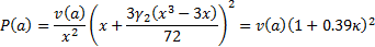
The physical interpretation of this is that, if these
assumptions apply, then the 1 in 200 quantile is a factor of  further into
the tail than we might otherwise expect purely from the standard deviation of
the distribution.
further into
the tail than we might otherwise expect purely from the standard deviation of
the distribution.
(b) Unfortunately, the 4th
order Cornish-Fisher expansion is not in general very good at estimating the
shape of the distributional form in regions in which we might be most
interested, see e.g. Kemp (2009).
In effect, the computation of skew and kurtosis gives ‘too much’ weight to the
extent of non-normality in the centre of the distributional form whereas
typically for risk management purposes we are most interested in the extent of
non-normality in the tail of the distribution. He proposes an alternative
approach, more directly akin to fitting a curve through the observed (ordered)
distributional form, to ‘extrapolate into the tail’.
Such an approach is more computationally
intensive than the Cornish-Fisher approach, particularly if the data series in
question involve a large number of terms. The approach requires the return
series to be sorted, in order to work out which observations to give most
weight to in the curve fitting algorithm. Sorting large data sets is
intrinsically much slower than merely calculating their moments since it
typically involves a number of computations that scales in line with
approximately  rather than
merely
rather than
merely  . It may be
that such a refinement would not in practice lead to a much enhanced risk
model, as non-zero kurtosis is still typically a good indicator of the presence
of fat-tailed behaviour, even if it is not a particularly good indicator of
exactly how fat-tailed it is in the particular part of the distributional form
in which we might be most interested.
. It may be
that such a refinement would not in practice lead to a much enhanced risk
model, as non-zero kurtosis is still typically a good indicator of the presence
of fat-tailed behaviour, even if it is not a particularly good indicator of
exactly how fat-tailed it is in the particular part of the distributional form
in which we might be most interested.
(c) More
problematic, perhaps, is another topic that Kemp explores in Kemp (2009) and
Kemp (2010).
He notes, as implicitly have earlier authors, that much of the fat-tailed
behaviour observed in practice in return series (both when viewed singly and
when viewed jointly) seems to derive from time-varying volatility, see Section
4.3.
NAVIGATION LINKS
Contents | Prev | Next