Clustering techniques for universe
selection
[this page | pdf | references | back links]
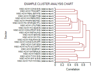
Example Cluster Analysis
(click on chart for more details)

1.
Cluster analysis is a well-established tool in quantitative
finance. We might for example want to know which stocks appear to behave most
‘similarly’ to which other stocks, thus grouping together stocks that appear to
have similar economic characteristics. Market index data vendors often classify
stocks according to some predefined industry classification, but not all stocks
easily fit into such classifications. Even if they did, which industry
sub-types should be grouped together to form overall industry sectors? Also, is
it better to analyse stocks by country first and then sector or vice-versa?
Etc.
2.
Most types of cluster analysis used in finance involve hierarchical
clustering. This can be thought of as a form of unsupervised learning.
We have some information about individual elements and we want to build up a
nested tree that best characterises the degree of linkage between the different
elements (without presupposing any ‘right answer’ in advance). For example, we
might have a series of stock or sector returns, and we want to see which ones
appear to be closest to each other. The output is a bunch of fully nested sets.
The smallest sets are the individual elements themselves. The largest set is
the whole data set. The intermediate sets are nested, i.e. the intersection of
any two sets is either the null set or the smaller of the two sets.
3.
The common convention is to have the nesting arrangement form a binary
tree, i.e. where each larger set is deemed to split into just two
sub-sets at each node of the tree. Where say three subsets are equally near
each other within a larger set then this is typically represented by an
arbitrary choice of one of the three subsets to stand distinct and for a branch
of zero length to join it to the join of the other two subsets.
4.
For example, quantitative equity research analysts might focus on
correlations between different regional sectors and correlations of stocks
within sectors, computed using regression analyses over over suitable rolling
periods, computing sector and country betas from the following formula, see
e.g. Morgan
Stanley (2002):

where:  is
return of stock
  in month
  ,
,  is
return of sector
  in month
  ,
,  is
return of country
  in month
  ,
,  and
and  are sector
and country of stock
  and
and  is
unexplained return of stock
  in month
5.
Precise choice of how to measure ‘degree of linkage’, i.e. the ‘distance’
between different elements, can be quite important in this context, and can
depend on what question we are trying to answer. For example, in an equity
orientated analysis as above, we might measure ‘distance’ either by reference
to correlations or by reference to covariances. If we use covariances then
relatively unvolatile stocks will be deemed to be relatively similar whilst
relatively volatile stocks may be deemed to be relatively different to each
other even when they are relatively highly correlated. The algorithm used to
derive the example cluster analysis shown above is based on one in Press et al.
(2007).
References
Morgan
Stanley (2002). Quantitative Strategies Research Note. Morgan Stanley
Press, W.H.,
Teukolsky, S.A., Vetterling, W.T. and Flannery, B.P. (2007). Numerical
Recipes: The Art of Scientific Computing. Cambridge University Press